
RNAseq DE analysis with R - Solutions
This document provides solutions to the exercises given in the ‘RNAseq DE analysis with R’ course.
Clustering
Exercise: Heatmap
Produce a heatmap for the 50 most highly expressed genes and annotate the samples with with their age.
- Subset the read counts object for the 30 most highly expressed genes
- Annotate the samples in the subset with their age (check order with design!)
- Plot a heatmap with this subset of data, scaling genes and ordering both genes and samples
Solution:
# Subset the read counts object for the 30 most highly expressed genes
select = order(rowMeans(counts$counts), decreasing=TRUE)[1:50]
highexprgenes_counts <- counts$counts[select,]

# Annotate the samples in the subset with their age (check order with design!)
colnames(highexprgenes_counts)<- experiment_design.ord$age
head(highexprgenes_counts)
## 26 26 30 30 30 26 26 30
## 4550 12559197 7221252 3612091 3696466 5332585 7045283 12201302 5190887
## 4549 2635341 1542503 880852 900136 1256473 1506197 2564452 1226882
## 213 711 633 1554756 1591787 1992909 541 560 1939249
## 378706 87658 2085194 1200456 1212964 62432 2063356 86078 61130
## 6029 44288 1461296 723247 726382 18142 1449540 43866 17747
## 125050 80094 740715 588378 595398 54657 726225 78199 53896# Plot a heatmap with this subset of data, scaling genes and ordering both genes and samples
heatmap(highexprgenes_counts, col=topo.colors(50), margin=c(10,6))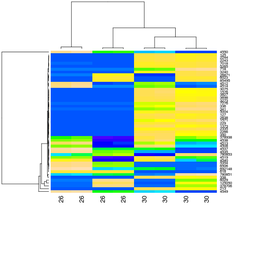
plot of chunk Heatmap
Principal Component Analysis
Exercise: PCA
Produce a PCA plot from the read counts of the 50 most highly expressed genes and change the labels until you can identify the reason for the split between samples from the same tissue.
- Get the read counts for the 50 most highly expressed genes
- Transpose this matrix of read counts
- Check the number of dimensions explaining the variability in the dataset
- Run the PCA with an appropriate number of components
- Annotate the samples with their age & re-run the PCA & plot the main components
- Annotate the samples with other clinical data & re-run the PCA & plot the main components until you can separate the samples within each tissue group
Solution:
library(mixOmics)## Loading required package: MASS
## Loading required package: lattice## Warning in rgl.init(initValue, onlyNULL): RGL: unable to open X11 display## Warning in fun(libname, pkgname): error in rgl_init# Get the read counts for the 50 most highly expressed genes
select = order(rowMeans(counts$counts), decreasing=TRUE)[1:50]
highexprgenes_counts <- counts$counts[select,]
# Transpose this matrix of read counts
data_for_mixOmics <- t(highexprgenes_counts)
# Check the number of dimensions explaining the variability in the dataset
tune = tune.pca(data_for_mixOmics, center = TRUE, scale = TRUE)## Eigenvalues for the first 8 principal components:
## PC1 PC2 PC3 PC4 PC5
## 3.287836e+01 1.507356e+01 2.030841e+00 1.555950e-02 8.432604e-04
## PC6 PC7 PC8
## 5.918977e-04 2.454588e-04 1.570937e-31
##
## Proportion of explained variance for the first 8 principal components:
##          PC1          PC2          PC3          PC4          PC5
## 6.575673e-01 3.014711e-01 4.061682e-02 3.111900e-04 1.686521e-05
##          PC6          PC7          PC8
## 1.183795e-05 4.909175e-06 3.141875e-33
##
## Cumulative proportion explained variance for the first 8 principal components:
## PC1 PC2 PC3 PC4 PC5 PC6 PC7
## 0.6575673 0.9590384 0.9996552 0.9999664 0.9999833 0.9999951 1.0000000
## PC8
## 1.0000000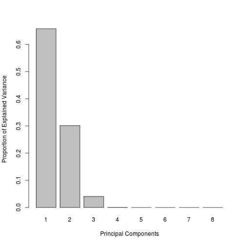
plot of chunk PCA
tune$prop.var## PC1 PC2 PC3 PC4 PC5
## 6.575673e-01 3.014711e-01 4.061682e-02 3.111900e-04 1.686521e-05
## PC6 PC7 PC8
## 1.183795e-05 4.909175e-06 3.141875e-33# Run the PCA with an appropriate number of components
result <- pca(data_for_mixOmics, ncomp = 3, center = TRUE, scale = TRUE)
plotIndiv(result, comp = c(1, 2), ind.names = TRUE) 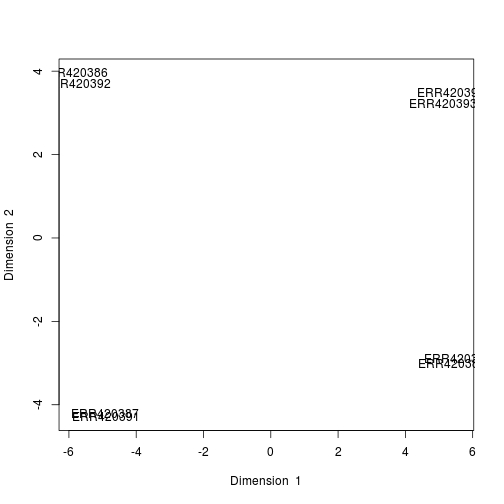
plot of chunk PCA
# Annotate the samples with their age \& re-run the PCA \& plot the main components
rownames(data_for_mixOmics)<- experiment_design.ord$age
result <- pca(data_for_mixOmics, ncomp = 3, center = TRUE, scale = TRUE)
plotIndiv(result, comp = c(1, 2), ind.names = TRUE) 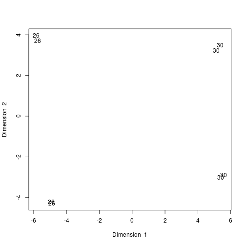
plot of chunk PCA
# Annotate the samples with other clinical data \& re-run the PCA \& plot the main components until you can separate the samples within each tissue group
rownames(data_for_mixOmics)<- experiment_design.ord$technical_replicate_group
result <- pca(data_for_mixOmics, ncomp = 3, center = TRUE, scale = TRUE)
plotIndiv(result, comp = c(1, 2), ind.names = TRUE) 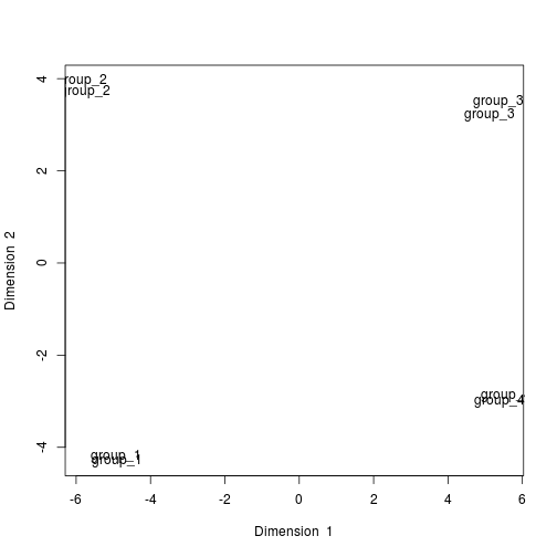
plot of chunk PCA
Differential Expression
Exercise: Limma
Get the number of DE genes between technical group 1 and technical group 2 (all Brain samples) with adj pvalue<0.01.
- Create a new design matrix for limma with the technical replicate groups
- Re-normalise the read counts with ‘voom’ function with new design matrix
- Fit a linear model on these normalised data
- Make the contrast matrix corresponding to the new set of parameters
- Fit the contrast matrix to the linear model
- Compute moderated t-statistics of differential expression
- Get the output table for the 10 most significant DE genes for this comparison
Solution:
library(limma)## Loading required package: methods# Create a new design matrix for limma with the technical replicate groups
techgroup<-factor(experiment_design.ord$technical_replicate_group)
design <- model.matrix(~0+techgroup)
colnames(design)<- gsub("techgroup","",colnames(design))
design## group_1 group_2 group_3 group_4
## 1 0 1 0 0
## 2 1 0 0 0
## 3 0 0 0 1
## 4 0 0 0 1
## 5 0 0 1 0
## 6 1 0 0 0
## 7 0 1 0 0
## 8 0 0 1 0
## attr(,"assign")
## [1] 1 1 1 1
## attr(,"contrasts")
## attr(,"contrasts")$techgroup
## [1] "contr.treatment"# Re-normalise the read counts with 'voom' function with new design matrix
y <- voom(mycounts,design,lib.size=colSums(mycounts)*nf)
counts.voom <- y$E
# Fit a linear model on these normalised data
fit <- lmFit(y,design)
# Make the contrast matrix corresponding to the new set of parameters
cont.matrix <- makeContrasts(group_2-group_1,levels=design)
cont.matrix ## Contrasts
## Levels group_2 - group_1
## group_1 -1
## group_2 1
## group_3 0
## group_4 0# Fit the contrast matrix to the linear model
fit <- contrasts.fit(fit, cont.matrix)
# Compute moderated t-statistics of differential expression
fit <- eBayes(fit)
options(digits=3)
# Get the output table for the 10 most significant DE genes for this comparison
dim(topTable(fit,coef="group_2 - group_1",p.val=0.01,n=Inf))## [1] 9652 6topTable(fit,coef="group_2 - group_1",p.val=0.01)## logFC AveExpr t P.Value adj.P.Val B
## 125050 -3.598 13.36 -1219 6.95e-58 1.04e-53 123.0
## 378706 -4.964 14.07 -842 4.15e-54 3.12e-50 114.4
## 6029 -5.432 13.07 -500 8.61e-49 4.31e-45 102.0
## 4514 0.761 12.20 271 1.44e-42 5.42e-39 86.5
## 26871 -2.795 10.87 -187 8.96e-39 2.69e-35 78.7
## 6023 -4.752 10.00 -168 1.16e-37 2.90e-34 76.5
## 6043 -2.923 8.73 -164 2.02e-37 4.34e-34 75.9
## 5354 0.576 5.73 158 4.82e-37 9.05e-34 74.3
## 692148 0.733 10.39 146 3.15e-36 5.26e-33 72.6
## 652965 -2.864 7.83 -137 1.36e-35 2.04e-32 71.6Gene Ontology
Exercise: GOstats
Identify the GO terms in the Molecular Function domain that are over-represented (pvalue<0.01) in your list of DE genes.
- Get your list of DE genes (Entrez Gene IDs)
- Set the new parameters for the hypergeometric test
- Run the test and adjust the pvalues in the output object
- Identify the significant GO terms at pvalue 0.01
Solution:
library(GOstats)## Loading required package: Biobase
## Loading required package: BiocGenerics
## Loading required package: parallel
##
## Attaching package: 'BiocGenerics'
##
## The following objects are masked from 'package:parallel':
##
## clusterApply, clusterApplyLB, clusterCall, clusterEvalQ,
## clusterExport, clusterMap, parApply, parCapply, parLapply,
## parLapplyLB, parRapply, parSapply, parSapplyLB
##
## The following object is masked from 'package:limma':
##
## plotMA
##
## The following object is masked from 'package:stats':
##
## xtabs
##
## The following objects are masked from 'package:base':
##
## anyDuplicated, append, as.data.frame, as.vector, cbind,
## colnames, do.call, duplicated, eval, evalq, Filter, Find, get,
## intersect, is.unsorted, lapply, Map, mapply, match, mget,
## order, paste, pmax, pmax.int, pmin, pmin.int, Position, rank,
## rbind, Reduce, rep.int, rownames, sapply, setdiff, sort,
## table, tapply, union, unique, unlist, unsplit
##
## Welcome to Bioconductor
##
## Vignettes contain introductory material; view with
## 'browseVignettes()'. To cite Bioconductor, see
## 'citation("Biobase")', and for packages 'citation("pkgname")'.
##
## Loading required package: Category
## Loading required package: stats4
## Loading required package: Matrix
## Loading required package: AnnotationDbi
## Loading required package: GenomeInfoDb
## Loading required package: S4Vectors
## Loading required package: IRanges
##
## Attaching package: 'IRanges'
##
## The following object is masked from 'package:Matrix':
##
## expand
##
##
## Attaching package: 'AnnotationDbi'
##
## The following object is masked from 'package:MASS':
##
## select
##
## Loading required package: GO.db
## Loading required package: DBI
##
## Loading required package: graph
##
## Attaching package: 'GOstats'
##
## The following object is masked from 'package:AnnotationDbi':
##
## makeGOGraph# Get your list of DE genes (Entrez Gene IDs)
entrezgeneids <- as.character(rownames(limma.res.pval.FC))
universeids <- rownames(mycounts)
# Set the new parameters for the hypergeometric test
params <- new("GOHyperGParams",annotation="org.Hs.eg",geneIds=entrezgeneids,universeGeneIds=universeids,ontology="MF",pvalueCutoff=0.01,testDirection="over")## Loading required package: org.Hs.eg.db## Warning in makeValidParams(.Object): removing geneIds not in
## universeGeneIds# Run the test and adjust the pvalues in the output object
hg <- hyperGTest(params)
hg.pv <- pvalues(hg)
hg.pv.fdr <- p.adjust(hg.pv,'fdr')
# Identify the significant GO terms at pvalue 0.01
sigGO.ID <- names(hg.pv.fdr[hg.pv.fdr < hgCutoff])
df <- summary(hg)
GOterms.sig <- df[df[,1] %in% sigGO.ID,"Term"]
length(GOterms.sig )## [1] 430head(GOterms.sig)## [1] "signaling receptor activity"
## [2] "transmembrane signaling receptor activity"
## [3] "signal transducer activity"
## [4] "molecular transducer activity"
## [5] "receptor activity"
## [6] "receptor binding"R environment
sessionInfo()## R version 3.2.0 (2015-04-16)
## Platform: x86_64-pc-linux-gnu (64-bit)
## Running under: Ubuntu 14.04.1 LTS
##
## locale:
## [1] LC_CTYPE=en_US.UTF-8 LC_NUMERIC=C
## [3] LC_TIME=en_US.UTF-8 LC_COLLATE=en_US.UTF-8
## [5] LC_MONETARY=en_US.UTF-8 LC_MESSAGES=en_US.UTF-8
## [7] LC_PAPER=en_US.UTF-8 LC_NAME=C
## [9] LC_ADDRESS=C LC_TELEPHONE=C
## [11] LC_MEASUREMENT=en_US.UTF-8 LC_IDENTIFICATION=C
##
## attached base packages:
## [1] stats4 parallel methods stats graphics grDevices utils
## [8] datasets base
##
## other attached packages:
## [1] org.Hs.eg.db_3.1.2 GOstats_2.34.0 graph_1.46.0
## [4] Category_2.34.2 GO.db_3.1.2 RSQLite_1.0.0
## [7] DBI_0.3.1 AnnotationDbi_1.30.1 GenomeInfoDb_1.4.1
## [10] IRanges_2.2.5 S4Vectors_0.6.1 Matrix_1.2-1
## [13] Biobase_2.28.0 BiocGenerics_0.14.0 limma_3.24.12
## [16] mixOmics_5.0-4 lattice_0.20-31 MASS_7.3-41
##
## loaded via a namespace (and not attached):
## [1] Rcpp_0.11.6 RGCCA_2.0 formatR_1.2
## [4] RColorBrewer_1.1-2 plyr_1.8.3 tools_3.2.0
## [7] annotate_1.46.0 evaluate_0.7 gtable_0.1.2
## [10] igraph_1.0.1 genefilter_1.50.0 stringr_1.0.0
## [13] knitr_1.10.5 grid_3.2.0 GSEABase_1.30.2
## [16] survival_2.38-2 XML_3.98-1.3 rgl_0.93.996
## [19] RBGL_1.44.0 pheatmap_1.0.2 magrittr_1.5
## [22] splines_3.2.0 scales_0.2.5 AnnotationForge_1.10.1
## [25] colorspace_1.2-6 xtable_1.7-4 stringi_0.5-5
## [28] munsell_0.4.2